
PARABOLA’S PARAMETERS
EFFECTS
By Dario Gonzalez
Everyone who is familiar with functions knows that the general equation for any quadratic functions is:
![]()
The idea now is to
explore the effects of each parameter ![]() and
and ![]() in the graph a quadratic function. First, we are going to review some basic
transformation when the quadratic function’s equation is written as follow:
in the graph a quadratic function. First, we are going to review some basic
transformation when the quadratic function’s equation is written as follow:
![]() Expression (1)
Expression (1)
It is precise to
emphasize that every quadratic function can be written as the Expression (1) by
following the completion of a square
method. That is, we can go from the
general expression to Expression (1) by doing as follow:
![]()
![]()
![]()
![]()
![]()
Here, we can consider:
![]() and
and ![]()
Then, we obtain the
Expression (1) again. This is a very
crucial fact since the Expression (1) can represent all the possible
transformation of the graph a quadratic function.
Given that most of you
are probably familiar with this fact, we will do a brief summary of the effects
produced by parameters ![]() and
and ![]() in the graph of the quadratic function.
in the graph of the quadratic function.
EFFECT OF PARAMETER ![]() :
:
If we consider the quadratic function
where the parameters ![]() and
and ![]() ,
and we make parameter
,
and we make parameter ![]() varies; by considering the function
varies; by considering the function ![]() as a reference, we will observe the effects of
parameter a in the graph of
as a reference, we will observe the effects of
parameter a in the graph of ![]() in the animation 1 below:
in the animation 1 below:
|
|
|
Animation 1 |
From figure 1 we can conclude the
effects of parameter ![]() if we consider as a reference the function
if we consider as a reference the function ![]() in the following table below:
in the following table below:
|
Sign of |
Positive |
Parabola is
opened upward |
|
Negative |
Parabola is
opened downward |
|
|
Value of |
|
Parabola
becomes broader |
|
|
Parabola
becomes steep |
EFFECTS
OF PARAMETER ![]() :
:
Now we are going to consider the quadratic function equation where
![]() and
and ![]() . That is, taking as a reference the function
. That is, taking as a reference the function ![]() , we can see the
graphic effects of parameter h in
, we can see the
graphic effects of parameter h in ![]() by observing the following animation 2:
by observing the following animation 2:
|
|
|
Animation 2 |
Then, we can summary the effects of
parameter ![]() in the table below:
in the table below:
|
Sign of |
Positive |
Right move |
|
Negative |
Left move |
EFFECTS
OF PARAMETER ![]() :
:
Finally, if we consider a quadratic
function whose parameters ![]() and
and ![]() and the function
and the function ![]() as a reference, we visualize the graphic
effect of parameter k for the function
as a reference, we visualize the graphic
effect of parameter k for the function ![]() in animation 3 below:
in animation 3 below:
|
|
|
Animation 3 |
Thus, we can summary the effects of
parameter ![]() in the table below:
in the table below:
|
Sign of |
Positive |
Move up |
|
Negative |
Move down |
In general, we can conclude that for
each function f(x) it is possible to make the following transformations:
|
Parameter |
Relationship |
Characteristic |
Graphic effect |
|
|
|
--------- |
Reflection
around of X axe of f(x) graph |
|
|
|
|
The images of
f(x) increase in a |
|
|
|
The images of
f(x) decrease in a |
|
|
|
|
Positive |
The graph of
f(x) moves right |
|
|
Negative |
The graph of
f(x) moves left |
|
|
|
|
Positive |
The graph of f(x)
moves up |
|
|
Negative |
The graph of
f(x) moves down |
Even though this explanation is enough
to solve problems from 1 through 6, I would like to offer a different
approach. This approach considers all
what we review before and the graphic sum.
GRAPHIC
SUM:
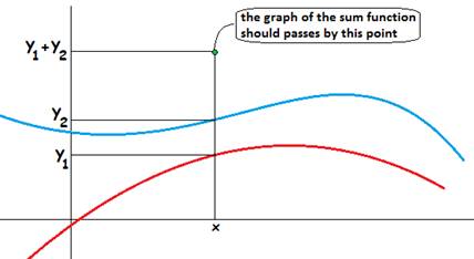
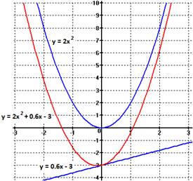
Graphic sum consists of obtaining the
graph of the sum function given the graphs of two functions. In other words, we consider the image of each
function in a fixed x, and we sum these two images obtaining one image if the
sum function for that fixed x. This
concept is shown in figure 1 below:
|
|
|
Figure 1 |
We must consider some important
observations:
Observation
1:
Let h(x) = f(x) + g(x), then h(x) = f(x) if g(x) = 0.
Observation
2:
Let h(x) = f(x) + g(x), then h(x) is going to behave like f(x) if |g(x)| is really small.
ANOTHER
APPROACH:
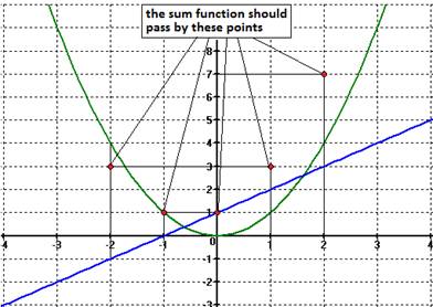
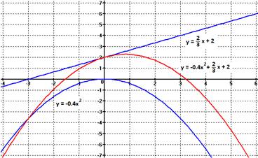
Consider the functions ![]() and
and ![]() whose graphs are shown in the figure 2 below:
whose graphs are shown in the figure 2 below:
|
|
|
Figure 2 |
We should highlight some important
issues in the sum of these two functions.
Issue
1: The sum function is going to intersect the linear function ![]() at x = 0, according to observation 1. Also, the sum function will behave similar to
linear function close to x = 0 because, according to observation2, the images
of the parabola are really small. It is important to note that the intersection
between the linear function and the sum function is tangential in x = 0. Indeed, if we analyze the values of the
functions f(x) and g(x) around x = 0,
we can see the values of the sum function will be slightly larger than the
linear function’s values. The only
exception occurs at x = 0 where both functions, the linear function and the sum
function, are equal.
at x = 0, according to observation 1. Also, the sum function will behave similar to
linear function close to x = 0 because, according to observation2, the images
of the parabola are really small. It is important to note that the intersection
between the linear function and the sum function is tangential in x = 0. Indeed, if we analyze the values of the
functions f(x) and g(x) around x = 0,
we can see the values of the sum function will be slightly larger than the
linear function’s values. The only
exception occurs at x = 0 where both functions, the linear function and the sum
function, are equal.
Issue
2: The images of ![]() are going to be much larger than the images of
are going to be much larger than the images of
![]() when the value of x goes to infinity; that is,
when
when the value of x goes to infinity; that is,
when ![]() the sum function will behave like a parabola
because the values of the linear function will be small in comparison to the
values of the parabola (observation 2).
the sum function will behave like a parabola
because the values of the linear function will be small in comparison to the
values of the parabola (observation 2).
Issue
3: Given the algebraic sum between ![]() and
and ![]() does not modify the coefficient of
does not modify the coefficient of ![]() , we can conclude
that the sum function, which is going to be another parabola, has the same breadth of
, we can conclude
that the sum function, which is going to be another parabola, has the same breadth of ![]() , according to
analysis of the parameters’ effects done above.
, according to
analysis of the parameters’ effects done above.
So, given the issues above mentioned,
the graph of the sum function is going to be a parabola like ![]() , but this sum
function will be tangent to the linear function
, but this sum
function will be tangent to the linear function ![]() in x = 0.
The graph of the sum function is shown below:
in x = 0.
The graph of the sum function is shown below:
|
|
|
Figure 3 |
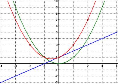
I plotted the graph of the sum
function with the graphs of the others function because I would like you to
appreciate how the sum graph has exactly the same shape that the parabola f(x),
but it is positioned on the linear
function ![]() .
.
Given that our above reasoning and
according to observation 2 and issue 1, we can conclude that even though the
green parabola could have been any parabola of the family ![]() , the sum
function would have had the same behavior.
In other words, it does not matter what is the value of parameter
, the sum
function would have had the same behavior.
In other words, it does not matter what is the value of parameter ![]() , if we do the
sum between
, if we do the
sum between ![]() and
and ![]() , we would have
obtained the same result; that is, the sum function will be a parabola like
, we would have
obtained the same result; that is, the sum function will be a parabola like ![]() , but it would
have been tangentially positioned on
the linear function
, but it would
have been tangentially positioned on
the linear function ![]() .
.
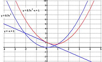
However, we can go further with this
conclusion. Observe the graphs shown in
figure 4. The blue graphs are the addend
functions, and the red graph is the sum function.
|
Figure 4 (a) |
|
|
Figure 4 (b) |
|
|
Figure 4 (c) |
|
After observing these graphs, we can
realize that the behavior of the sum function between a parabola ![]() and a linear function
and a linear function ![]() could be generalized in the following
statement:
could be generalized in the following
statement:
Statement
1: Given a parabola ![]() and a linear function
and a linear function ![]() , the graph of
the function h(x) = f(x) + g(x) is a parabola like
, the graph of
the function h(x) = f(x) + g(x) is a parabola like ![]() , but its graph
will be tangentially positioned on
the linear function
, but its graph
will be tangentially positioned on
the linear function ![]() in x = 0.
In other words,
in x = 0.
In other words, ![]() is a parabola tangent to
is a parabola tangent to ![]() at x = 0.
at x = 0.
That statement establishes a crucial
base for our analysis about of the effects of the parameters ![]() and
and ![]() in the graph of the quadratic function
in the graph of the quadratic function ![]() . That is, we could consider the quadratic
function h(x) as a sum of two functions
. That is, we could consider the quadratic
function h(x) as a sum of two functions ![]() and
and ![]() , and from this
assumption, we can draw a interesting analysis of the parameters
, and from this
assumption, we can draw a interesting analysis of the parameters ![]() and
and ![]() .
.
EFFECTS
OF PARAMETERS ![]() AND
AND ![]() :
:
The analysis developed above will
allow us to examine the graphic effects of the parameters ![]() and
and ![]() in the quadratic function
in the quadratic function ![]() .
.
1) Parameter ![]() : First of all, by
appreciating figure 4 (a), (b) and (c), we reason that the parameter
: First of all, by
appreciating figure 4 (a), (b) and (c), we reason that the parameter ![]() has two graphic representations: on the one
hand,
has two graphic representations: on the one
hand, ![]() represents the y-intersection for
represents the y-intersection for ![]() . On the other hand,
. On the other hand, ![]() determines the tangential intercept point
between the linear function
determines the tangential intercept point
between the linear function ![]() and the quadratic function
and the quadratic function ![]() .
.
It is effortless to reach the anterior
conclusion if we consider the function ![]() as sum of
as sum of ![]() and
and ![]() . We know the parameter
. We know the parameter ![]() in the linear function g(x) represents the
y-intercept, which occurs at x = 0 because
in the linear function g(x) represents the
y-intercept, which occurs at x = 0 because ![]() . Also, we know that
. Also, we know that ![]() , then
, then ![]() . Thus,
. Thus, ![]() also represents the y-intersection for h(x).
also represents the y-intersection for h(x).
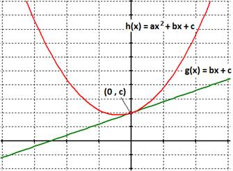
Moreover, we show easily that the
interception between h(x) and g(x) is tangential and occurs at
![]() . To find the interceptions between h(x) and
g(x) we must solve the equation:
. To find the interceptions between h(x) and
g(x) we must solve the equation:
![]()
![]()
![]()
So, there exist exactly one
intersection between h(x) and g(x) that occurs at x = 0, and, given that ![]() , this intersection
appears at
, this intersection
appears at ![]() .
.
|
|
|
Figure 5 |
You can observe the following
animation 4 to visualize graphically the effects of parameter c.
|
|
|
Animation 4 |
2) Parameter ![]() : Recall statement
1 and issue 3, we are capable to examine the graphic effect of parameter
: Recall statement
1 and issue 3, we are capable to examine the graphic effect of parameter ![]() . The graph of a quadratic function
. The graph of a quadratic function ![]() is just a translation of the graph of the parabola
is just a translation of the graph of the parabola ![]() . How we already know, h(x) is tangent to g(x)
at x = 0, then
. How we already know, h(x) is tangent to g(x)
at x = 0, then ![]() must have slope
must have slope ![]() at x = 0.
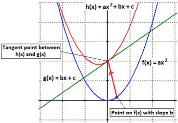
Thus, h(x) is the translation of
at x = 0.
Thus, h(x) is the translation of ![]() in a way that the point with slope
in a way that the point with slope ![]() on f(x) must intercept g(x)
at
on f(x) must intercept g(x)
at ![]() .
.
|
|
|
Figure 6 |
If we make parameter ![]() varies and fix parameters
varies and fix parameters ![]() and
and ![]() , the slope of
g(x) is going to change, and the graph of g(x) is going to act as a seesaw.
So, given that h(x) is tangent to g(x) at x = 0, we can visualize the
graph of h(x) seems to glide along the linear function g(x) as follow
in animation 5 below:
, the slope of
g(x) is going to change, and the graph of g(x) is going to act as a seesaw.
So, given that h(x) is tangent to g(x) at x = 0, we can visualize the
graph of h(x) seems to glide along the linear function g(x) as follow
in animation 5 below:
|
|
|
Animation 5 |
This effect of the parameter ![]() rest upon the fact that the slope of
rest upon the fact that the slope of ![]() only depend of this parameter when
only depend of this parameter when ![]() . In other words, the instantaneous change rate
of h(x) is
. In other words, the instantaneous change rate
of h(x) is ![]() when
when ![]() . Hence,
. Hence,
![]()
![]()
Thus,
![]()
Therefore, the parabola h(x) moves along the linear function g(x)
because the parabola h(x) has to keep tangentially touching g(x) at ![]() .
.
3) Parameter ![]() : We already know that the graph of a parabola
: We already know that the graph of a parabola ![]() represents a translation of the graph of a
parabola
represents a translation of the graph of a
parabola ![]() such that the point on the graph of f(x) that
has slope
such that the point on the graph of f(x) that
has slope ![]() is translated to be a tangential intersection
with the liner function
is translated to be a tangential intersection
with the liner function ![]() at x = 0.
Thus, we can analyze the effects of the parameter
at x = 0.
Thus, we can analyze the effects of the parameter ![]() by observing the effects in
by observing the effects in ![]() , which we
already did, and considering the relationship above explained between h(x) and
g(x).
, which we
already did, and considering the relationship above explained between h(x) and
g(x).
The parameter ![]() modifies the breadth and the orientation of
modifies the breadth and the orientation of ![]() like it was shown in figure 1. Consider
like it was shown in figure 1. Consider ![]() to be positive and vary whereas we fix the
other parameters
to be positive and vary whereas we fix the
other parameters ![]() and
and ![]() . As we know, the breadth of the parabola f(x)
will change, and given that the statement 1 still holds, the effects of
parameter
. As we know, the breadth of the parabola f(x)
will change, and given that the statement 1 still holds, the effects of
parameter ![]() on the graph of
on the graph of ![]() can be described as an up-down movement around
the liner function g(x). That is, when
can be described as an up-down movement around
the liner function g(x). That is, when ![]() h(x) becomes broader and moves down around the
linear function g(x). If
h(x) becomes broader and moves down around the
linear function g(x). If ![]() h(x) becomes steep and moves up around he
linear function g(x). This is shown in
the animation 6 below:
h(x) becomes steep and moves up around he
linear function g(x). This is shown in
the animation 6 below:
|
|
|
Animation 6 |
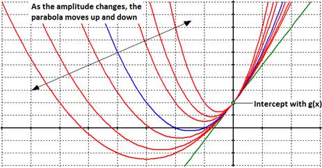
Here, in figure 7 below, there is a sort of a summary picture that shows a comparison among parabolas that have
different values for parameter a. The graph reference is the graph of ![]() , which is
presented by the blue parabola.
, which is
presented by the blue parabola.
|
|
|
Figure 7 |
Now if we consider ![]() negative, and we have
negative, and we have ![]() then the parabola h(x) becomes broader and
move up around the liner function g(x).
If
then the parabola h(x) becomes broader and
move up around the liner function g(x).
If ![]() then the parabola h(x) becomes steep and moves
down around the liner function g(x).
This is shown is animation 7 below:
then the parabola h(x) becomes steep and moves
down around the liner function g(x).
This is shown is animation 7 below:
|
|
|
Animation 7 |
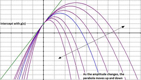
Here, in figure 8 below, there is a sort of a summary picture that shows a comparison among parabolas that have
different values for parameter a (now for negative values). The graph reference is the graph of ![]() , which is
presented by the blue parabola.
, which is
presented by the blue parabola.
|
|
|
Figure 8 |
Of course,
if parameter a = 0 the parabola becomes into a linear function
and, for this case, the “linear” parabola coincides with the linear function g(x)
= bx + c.
FINAL COMMENTS
I would like to highlight some final comments according to what we
have been analyzing here.
Comment 1: The functions ![]() and
and ![]() have the same value for their first derivative
at x = 0.
have the same value for their first derivative
at x = 0.
Comment 2: The function ![]() will have a root at x = 0 if and only if c =
0.
will have a root at x = 0 if and only if c =
0.
Comment 3: The vertex of
the function ![]() will be the intersection point with the linear
function
will be the intersection point with the linear
function ![]() if and only if b = 0.
if and only if b = 0.
